


Dithering With Quantization to Smooth Things Over
It should probably come as no surprise to anyone that the images which we look at every day – whether printed or on a display – are simply illusions. That cat picture isn’t actually a cat, but rather a collection of dots that when looked at from far enough away tricks our brain into thinking that we are indeed looking at a two-dimensional cat and happily fills in the blanks. These dots can use the full CMYK color model for prints, RGB(A) for digital images or a limited color space including greyscale.
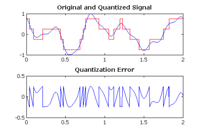
Perhaps more interesting is the use of dithering to further trick the mind into seeing things that aren’t truly there by adding noise. Simply put, dithering is the process of adding noise to reduce quantization error, which in images shows up as artefacts like color banding. Within the field of digital audio dithering is also used, for similar reasons. Part of the process of going from an analog signal to a digital one involves throwing away data that falls outside the sampling rate and quantization depth.
By adding dithering noise these quantization errors are smoothed out, with the final effect depending on the dithering algorithm used.
The Digital Era
Plot of a quantized signal and its error. (Source: Wikimedia)
For most of history, humanity’s methods of visual-auditory recording and reproduction were analog, starting with methods like drawing and painting. Until fairly recently reproducing music required you to assemble skilled artists, until the arrival of analog recording and playback technologies. Then suddenly, with the rise of computer technology in the second half of the 20th century we gained the ability to not only perform analog-to-digital conversion, but also store the resulting digital format in a way that promised near-perfect reproduction.
Digital optical discs and tapes found themselves competing with analog formats like the compact cassette and vinyl records. While video and photos remained analog for a long time in the form of VHS tapes and film, eventually these all gave way to the fully digital world of digital cameras, JPEGs, PNGs, DVDs and MPEG. Despite the theoretical pixel- and note-perfect reproduction of digital formats, considerations like sampling speed (Nyquist frequency) and the aforementioned quantization errors mean a range of new headaches to address.
That said, the first use of dithering was actually in the 19th century, when newspapers and other printed media were looking to print phots without the hassle of having a woodcut or engraving made. This led to the invention of halftone printing.
Polka Dots
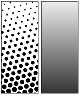
Left: halftone dot pattern with increasing size downwards, Right: how the human eye would see this, when viewed from a sufficient distance. (Source: Wikimedia)
With early printing methods, illustrations were limited to an all-or-nothing approach with their ink coverage. This obviously meant serious limitations when it came to more detailed illustrations and photographs, until the arrival of the halftone printing method. First patented in 1852 by William Fox Talbot, his approach used a special screen to break down an image into discrete points on a photographic plate. After developing this into a printing plate, these plates would then print this pattern of differently sized points.
Although the exact halftone printing methods were refined over the following decades, the basic principle remains the same to this day: by varying the size of the dot and the surrounding empty (white) space, the perceived brightness changes. When this method got extended to color prints with the CMYK color model, the resulting printing of these three colors as adjoining dots allowed for full-color photographs to be printed in newspapers and magazines despite having only so few ink colors available.
While it’s also possible to do CMYK printing with blending of the inks, as in e.g. inkjet printers, this comes with some disadvantages especially when printing on thin, low-quality paper, such as that used for newspapers, as the ink saturation can cause the paper to rip and distort. This makes CMYK and monochrome dithering still a popular technique for newspapers and similar low-fidelity applications.
Color Palettes
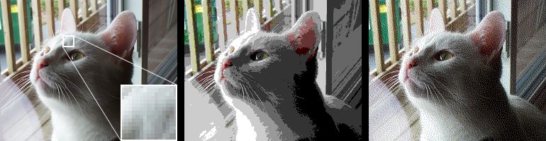
In an ideal world, every image would have an unlimited color depth. Unfortunately we sometimes have to adapt to a narrower color space, such as when converting to the Graphics Interchange Format (GIF), which is limited to 8 bits per pixel. This 1987-era and still very popular format thus provides an astounding 256 possible colors -albeit from a full 24-bit color space – which poses a bit of a challenge when using a 24-bit PNG or similar format as the source. Simply reducing the bit depth causes horrible color banding, which means that we should use dithering to ease these sharp transitions, like the very common Floyd-Steinberg dithering algorithm:
From left to right: original image. Converted to web safe color. Web safe with Floyd-Steinberg dithering. (Source: Wikipedia)
The Floyd-Steinberg dithering algorithm was created in 1976 by Robert W. Floyd and Louis Steinberg. Its approach to dithering is based on error diffusion, meaning that it takes the quantization error that causes the sharp banding and distributes it across neighboring pixels. This way transitions are less abrupt, even if it means that there is noticeable image degradation (i.e. noise) compared to the original.
This algorithm is quite straightforward, working its way down the image one pixel at a time without affecting previously processed pixels. After obtaining the current pixel’s quantization error, this is distributed across the subsequent pixels following and below the current one, as in the below pseudo code:
for each y from top to bottom do
for each x from left to right do
oldpixel := pixels[x]
[y] newpixel := find_closest_palette_color(oldpixel)
pixels[x][y] := newpixel
quant_error := oldpixel - newpixel
pixels[x + 1][y ] := pixels[x + 1][y ] + quant_error × 7 / 16
pixels[x - 1][y + 1] := pixels[x - 1][y + 1] + quant_error × 3 / 16
pixels[x ][y + 1] := pixels[x ][y + 1] + quant_error × 5 / 16
pixels[x + 1][y + 1] := pixels[x + 1][y + 1] + quant_error × 1 / 16
The implementation of the find_closest_palette_color() function is key here, with for a greyscale image a simple round(oldpixel / 255) sufficing, or trunc(oldpixel + 0.5) as suggested in this CS 559 course material from 2000 by the Universe of Wisconsin-Madison.
As basic as Floyd-Steinberg is, it’s still commonly used today due to the good results that it gives with fairly minimal effort. Which is not to say that there aren’t other dithering algorithms out there, with the Wikipedia entry on dithering helpfully pointing out a number of alternatives, both within the same error diffusion category as well as other categories like ordered dithering. In the case of ordered dithering there is a distinct crosshatch pattern that is both very recognizable and potentially off-putting.
Dithering is of course performed here to compensate for a lack of bit-depth, meaning that it will never look as good as the original image, but the less obnoxious the resulting artefacts are, the better.
Dithering With Audio
Although at first glance dithering with digital audio seems far removed from dithering the quantization error with images, the same principles apply here. When for example the original recording has to be downsampled to CD-quality (i.e. 16-bit) audio, we can either round or truncate the original samples to get the desired sample size, but we’d get distortion in either case. This distortion is highly noticeable by the human ear as the quantization errors create new frequencies and harmonics, this is quite noticeable in the 16- to 6-bit downsampling examples provided in the Wikipedia entry.
In the sample with dithering, there is clearly noise audible, but the original signal (a sine wave) now sounds pretty close to the original signal. This is done through the adding of random noise to each sample by randomly rounding up or down and counting on the average. Although random noise is clearly audible in the final result, it’s significantly better than the undithered version.
Random noise distribution is also possible with images, but more refined methods tend to give better results. For audio processing there are alternative noise distributions and noise shaping approaches.
Regardless of which dither method is being applied, it remains fascinating how the humble printing press and quantization errors have led to so many different ways to trick the human eye and ear into accepting lower fidelity content. As many of the technical limitations that existed during the time of their conception – such as expensive storage and low bandwidth – have now mostly vanished, it will be interesting to see how dithering usage evolves over the coming years and decades.
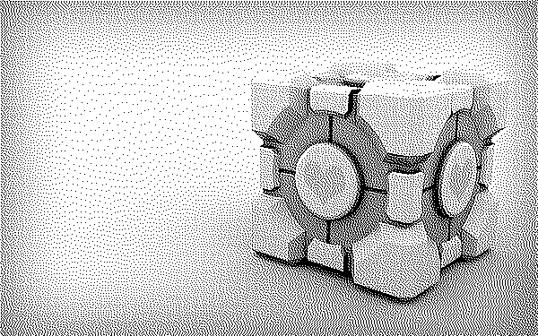
Featured image: “JJN Dithering” from [Tanner Helland]’s great dithering writeup.